A solution is a tree, not a line

When people write an ARC solution, it usually looks like a straight line of steps:

def solve_0520fde7(I):
    x1 = vmirror(I)
    x2 = lefthalf(x1)
    x3 = righthalf(x1)
    x4 = vmirror(x3)
    x5 = cellwise(x2, x4, ZERO)
    O  = replace(x5, ONE, TWO)
    return O

Six lines, top to bottom. It reads as a sequence. But that’s an artifact of how we write code, not the shape of the thing. Trace the data flow and the same solution is a tree (a DAG, really): vmirror branches into lefthalf and righthalf, those flow back together at cellwise, and constants like ZERO, ONE, TWO feed in from the side.

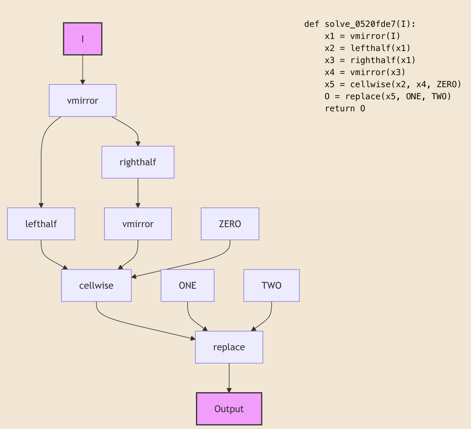
solve_0520fde7 as code and as a tree. The linear program is just one serialization of this branching structure.

I think this matters because human thinking isn’t sequential either — it’s more tree- or graph-shaped, with sub-results that get combined. So the natural representation of a solution is a tree: transformations as internal nodes, operands as leaves (input grids, constants, extracted properties).

And it’s not only the transformation that’s a tree. The condition that decides when a rule should fire is one too. A realistic firing condition is a nested pile of logic:

(((A or B or C) and D and E) or (F and G and H)) and ... and O

which is naturally a tree with AND/OR as internal nodes and property tests as leaves:

AND
├── OR
│   ├── AND ── (A or B or C), D, E
│   └── AND ── F, G, H
└── ...
        A = { size.height   == 1 }
        D = { symmetry.hori  == true }
        J = { shape          == "rectangle" }

So both halves of a rule — the what (transformation) and the when (condition) — want to be trees.

Here’s why I find that exciting rather than just tidy. Once a solution is a tree, you can compare two solutions by comparing their trees. If two different tasks are solved by structurally similar trees, they very likely share an underlying abstraction. And “the shared part of two trees” is not a vague idea — it’s a precise operation: find the largest common skeleton of both trees and leave the parts that differ as variables.

That operation has a name. It’s anti-unification — the dual of unification — introduced by Plotkin (1970) and Reynolds the same year, which computes the least general generalization of two terms (for a modern tour, see Cerna and Kutsia’s 2023 survey). It is, almost literally, the formal version of the question “what do these two solutions have in common?” — the same commonality-finding move I keep coming back to, but lifted from grids to programs.

I’m not claiming my system does this yet. But this is the bridge I keep seeing in the distance, and it’s why I care about getting the representation right first:

represent solutions and conditions as trees → compare the trees → generalize the shared skeleton by anti-unification → accumulate those skeletons as reusable abstractions.

Get a line of code to admit it’s a tree, and suddenly “learning a general rule from two examples” turns into a concrete tree operation. That’s the thread I’m pulling next.